4/29/2026

Optimizing Data Product Dependencies with Linear Programming

In the introductory blog post about Data Mesh as a Service, we discovered one particular challenge to optimize upstream dependencies. This time, we want to take a closer look at how to tackle this issue. But first let us revisit the problem in more detail.

What are upstream dependencies and why should we bother?

In the realm of data products, there are more often than not layers of them. In the well-known medallion architecture for instance, you will start out with raw data in the Bronze layer, clean and validate it in Silver and finally provide consumption-ready reports in Gold. This in turn means that any data product in Gold will have one or more upstream dependencies to data products in Silver which again are dependent on data products in Bronze.

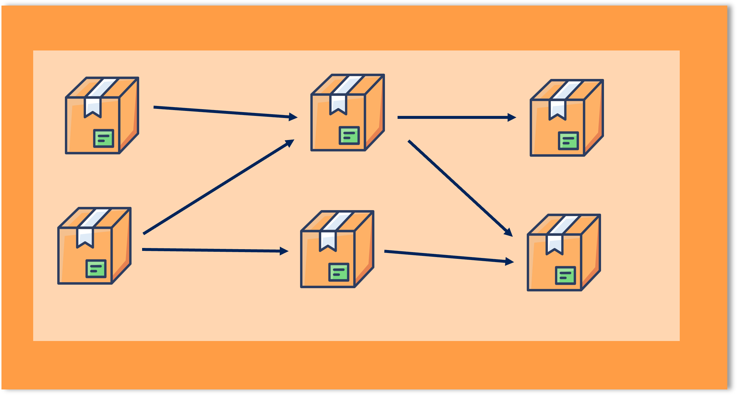
The image below shows a simple example of three layers of data products; arrows show data flow. Assuming these three layers to be bronze, silver and gold from left to right, we see two gold products. One of them has a single direct dependency to a silver product, which in turn depends on both bronze products. The other gold product, on the other hand has two direct dependencies on both silver products and also depends indirectly on both bronze products.

Dependencies in Data Products

While there is no way around such dependencies, we want to reduce coupling of data products and make them as coherent as possible. In other words, a data product should serve a single purpose but serve it well. This way, any dependency to a coherent data product will be well justified and make use of it as a whole. As a counterexample, assume that you create a single data product with all of your raw data in it. Now every single data product in Silver will have a dependency to your one and only Bronze data product. On the consumer side, this means you have to deal with a lot of unnecessary mental load. Furthermore, any change of your single upstream dependency might affect you. Even though, you only use a fraction of the data product, you will need to painstakingly check with every change, whether the part relevant to you was involved in the update.

Recall that we are working on so-called Managed Data Products that are used by different companies on their respective platform. In this case, having misaligned dependencies becomes suddenly much more expensive - quite literally. Not only do different customers have to deal with the already mentioned disadvantages of bloated products, they additionally will also need to load and compute data they do not really need, simply because it “came with the package”.

Problem Setting

When we started out creating managed data products, we had two things ready: working data marts from the existing data warehouses and an extensive analysis, which tables from the source database are being used in which data marts. Our initial plan was pretty simple - put every data mart into a separate gold data product and group source tables into sensible bronze products to optimize dependencies. Notice that silver is missing in this picture, but making sure that raw source tables are already in optimized packages will help us in any case.

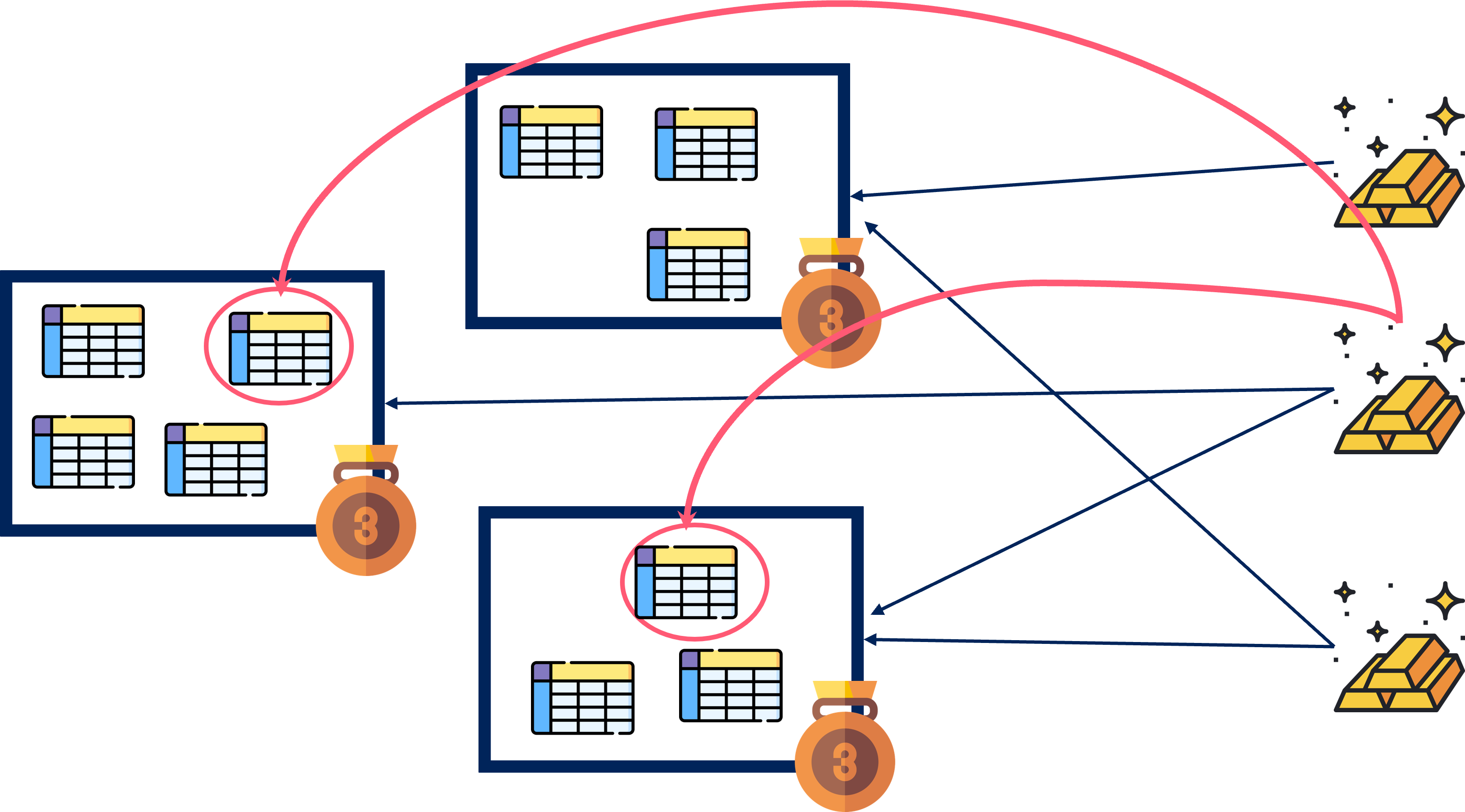
The picture below shows an example we are trying to avoid. There are three gold product with dependencies - displayed as the black arrows - to the bronze products. Each bronze product is essentially a collection of source tables. While the gold product in the middle depends on two different bronze products, it actually only uses one table of each. Thus, in the worst case, the gold product will require a customer to load seven tables while only using two of them.

Inefficient Dependencies

Linear Programming to the Rescue!

A pretty neat way to maximize or minimize a target with certain constraints is Linear Programming (LP). As stated in the name, the only requirement to use this approach is that both the target and the constraints can be expressed as linear relationships. But let us make it more accessible with a small example.

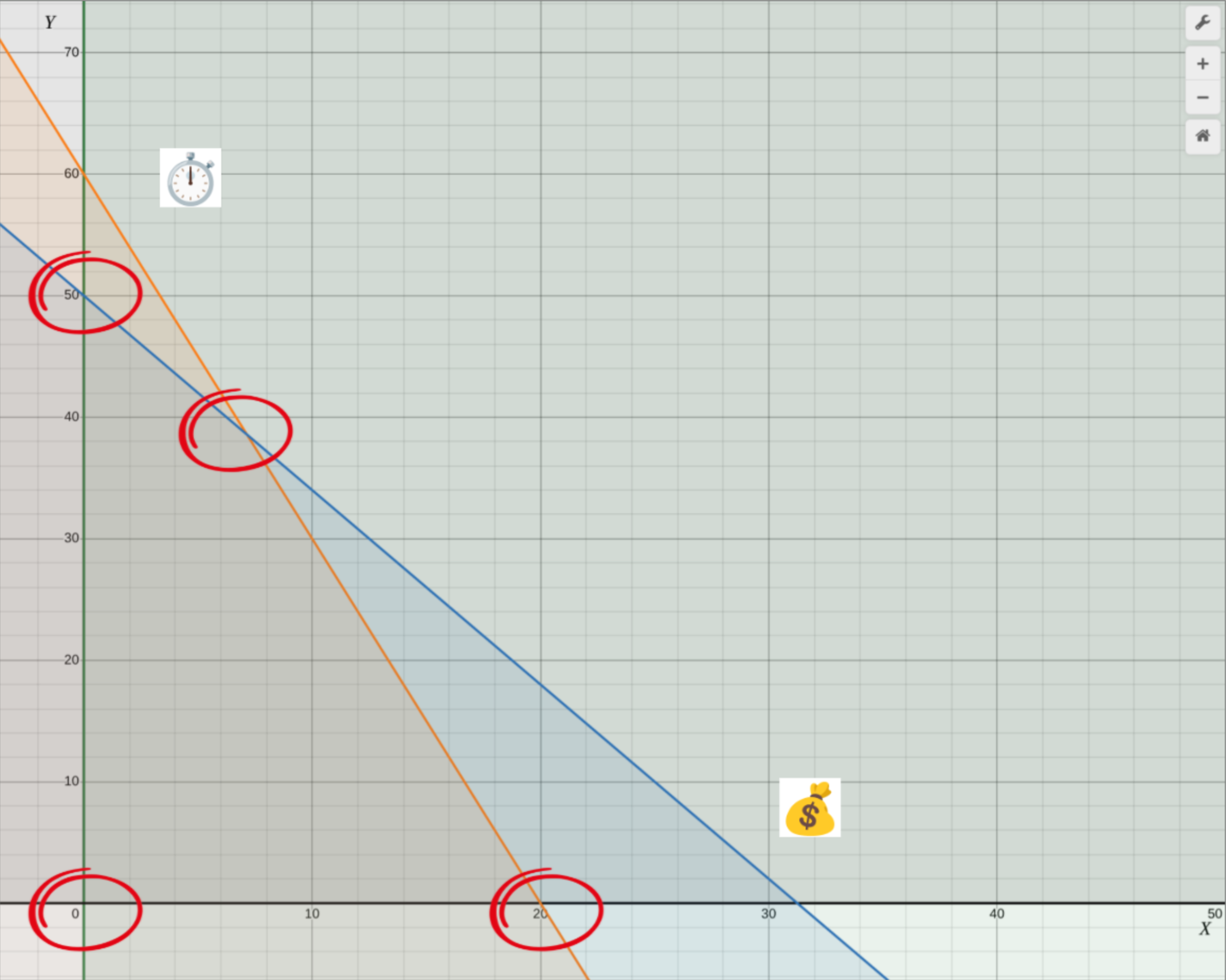
Assume you are the head of a manufacturing plant. Your plant produces both balls and sticks for sports. Both of these articles use up a certain amount of your resources (measured in money) and require time of your employees to actually produce them (measured in hours). Assume a ball requires 3 hours time and 8$ worth of materials, while a stick can be made within an hour from 5$ worth of resources. You have 60 hours and a budget of 250$ for this week’s production. You can sell balls for 20$ a piece; sticks can be sold for 10. Which items should be produced in which quantities to optimize your earnings?

This example problem can be expressed with linear inequalities as follows.

\begin{alignat*}{3} \max \quad 20x &+ 10 y \\ \text{subject to} \quad 3x &+ 1y \quad &\leq \quad &60 \\ 8x &+ 5y &\leq \quad &250 \\ x &&\geq \quad &0\\ y &&\geq \quad &0 \\ \end{alignat*}

Since this problem only uses two variables (the number of balls and sticks), we can also display the system and its possible solutions in a Cartesian graph. The solution will be found in one of the corner points and can be computed to gain a profit of exactly 528.57$. Unfortunately, standard algorithms assume variables to be a floating point number, which translates badly to units of balls and sticks. But we will not dive into this issue for the time being.

Graph of Example Problem

In the next section we will now apply this approach to find bronze products that optimize downstream dependencies.

Modelling the Data Product Dependency Problem

Getting back to our original question, we now need to formalize constraints and an optimization goal that express the need for efficient dependencies from gold products to bronze products. The biggest challenge might be defining variables that make meaningful statements possible in the first place. For this purpose we will use binary variables, which can only have two different values - 0 or 1. Such variables are used to model decisions essentially saying that whatever statement the variable models is true or false.

More precisely, we will use two types of variables: $gb_{i,j}$ is 1 if and only if gold product $i$ uses bronze product $j$ , $bt_{k,l}$ is 1 if and only if bronze product $k$ contains source table $l$ . Notice that we will have many more variables as in our example problem. Assuming there are 10 source tables, 10 bronze data products and 5 gold data products. We will have a hundred variables describing which source table is in which bronze product ( $bt_{k,l}$ ) and 50 variables for dependencies of gold products to bronze products ( $gb_{i,j}$ ). As an example: $bt_{1,5} = 1$ means that bronze data product 1 contains source table 5.

You are probably wondering now what source table 5 might be. Of course, source tables usually have more descriptive names. However, for the sake of shorter variable names we enumerate them. Since we know already all of our source tables and gold data products we can easily assign each one a number. This operation is a bit more involved when it comes to bronze product. Remember that we want to define nice and tidy bronze products in the first place, so how should we enumerate them? The simple solution is to just guess. If we find 20 bronze products a reasonable number, we can define the variables accordingly and let the computation run. If we are not satisfied with the result, we can still start a second run with more or less bronze products.

After all of these preparations, we are now finally able to set up the linear system.

\begin{alignat*}{2} \min &\sum_{ijk} t_k \cdot gb_{ij}\cdot bt_{jk} \quad \\ \text{subject to} \quad \forall_j \ &\sum_ibt_{ij} &= 1 \\ \forall_i \ &\sum_jbt_{ij} &\leq 5 \\ \forall_{\text{i,k where gold i requires table k}} \ &\sum_jgb_{ij}\cdot bt_{jk} &\geq 1 \\ \end{alignat*}

The linear system consists of a minimization goal and three constraints. The goal computes all tables that are being used by dependencies and multiplies them with a constant $t_k$ that indicates the size of source table $k$ . This value could either be the number of rows or its physical size in MB and works as a penalty for your solution that you want to keep as low as possible. The first constraint makes sure, that every source table is part of exactly one bronze product while the second constraint makes sure to have no more than five source tables per bronze product. The last constraint is the most essential one - it guarantees that all required dependencies from gold products to source tables are satisfied within configuration found.

Computing Solutions

Especially when the linear system gets large and we use special types of variables (such as binary or integer ones), we probably do not want to solve it ourselves. Luckily, there are countless numbers of open-source and proprietary solvers available. As a matter of fact, there are so many solvers that integrating a specific one to solve your problem is actually the wrong choice. Instead there are intermediaries such as pulp. They use an adapter pattern and make it possible for you to exchange the underlying solver for your problem on the go. In the problem above I noticed quickly that I might not find a perfect solution in reasonable time. At this point, I was quite happy that I was able to switch to a solver that also records intermediate, non-optimal solutions with barely any effort at all.

If you are eager to test it for yourself, you can find Jupyter Notebooks for both of the problems discussed in my repository.

Takeaway

We managed to optimize our dependencies by using linear programming. However, this tale is only just starting. The model we came up with so far is simple at best and there is still much potential for even more efficient data products! Here are just a few examples of what other aspects we could factor in to optimally group data into products:

Data sensitivity classification
Business domains
Source Systems

Furthermore, there are many more applications for this kind of approach outside of data dependency issues and I strongly encourage you to try it the next time you need to optimize something.